Predicting House Sale Prices in Boston

Based on the Boston, Ames housing dataset, I predicted sale price by shortlisting top explanatory variables from over 80 categorical, ordinal, discrete and continuous variables using correlation.
Read the code on Github here
Model Prediction of Housing Sale Price
Executive Summary
When it comes to housing prices, we often have access to extensive past data around housing features and the eventual sale price. Being able to predict future sale prices within a reasonable margin would be incredibly useful to many stakeholders, including housing agents, governing bodies and even residents themselves.
In this project, we process the Ames train and test datasets obtained via the Kaggle competition hosted by General Assembly to find a robust model based on 25-30 variables for prediction of house sale price. We look at which features affect sale price the most through data cleaning and exploratory data analysis, and build and refine our model using various regression techniques.
The data documentation for the original dataset can be viewed here.
Problem Statement
What features of a house contribute most significantly to its eventual sale price, and with knowledge of these features, how can we predict future sale price? Can the model that we build be generalised to other cities, states and countries?
We approach the problem statement from the POV of a team of housing agents in Ames, Iowa, as it’s likely that agents will have access to this level of detail about a property. Having a model will help agents to consistently valuate properties and negotiate better between buyers and sellers. If successful, this model could also then be marketed to both governing bodies and housing agents who would be interested in such a tool.
Approach
1. Data Cleaning & EDA
Data Description
The data dictionary below lists the variables that are available in this dataset and their definitions, per the original data documentation. The feature names used were changed to lowercase.
| Feature | Variable type | Datatype | Description |
|---|---|---|---|
| id | Discrete | int | Observation number |
| pid | Nominal | int | Parcel identification number |
| ms_subclass | Nominal | int | Identifies the type of dwelling involved in the sale |
| ms_zoning | Nominal | object | Identifies the general zoning classification of the sale |
| lot_frontage | Continuous | float | Linear feet of street connected to property |
| lot_area | Continuous | int | Lot size in square feet |
| street | Nominal | object | Type of road access to property |
| alley | Nominal | object | Type of alley access to property |
| lot_shape | Ordinal | object | General shape of property |
| land_contour | Nominal | object | Flatness of the property |
| utilities | Ordinal | object | Type of utilities available |
| lot_config | Nominal | object | Lot configuration |
| land_slope | Ordinal | object | Slope of property |
| neighborhood | Nominal | object | Physical locations within Ames city limits |
| condition_1 | Nominal | object | Proximity to various conditions |
| condition_2 | Nominal | object | Proximity to various conditions (if more than one is present) |
| bldg_type | Nominal | object | Type of dwelling |
| house_style | Nominal | object | Style of dwelling |
| overall_qual | Ordinal | int | Rates the overall material and finish of the house |
| overall_cond | Ordinal | int | Rates the overall condition of the house |
| year_built | Discrete | int | Original construction date |
| year_remod/add | Discrete | int | Remodel date (same as construction date if no remodeling or additions) |
| roof_style | Nominal | object | Type of roof |
| roof_matl | Nominal | object | Roof material |
| exterior_1st | Nominal | object | Exterior covering on house |
| exterior_2nd | Nominal | object | Exterior covering on house (if more than one material) |
| mas_vnr_type | Nominal | object | Masonry veneer type |
| mas_vnr_area | Continuous | float | Masonry veneer area in square feet |
| exter_qual | Ordinal | object | Evaluates the quality of the material on the exterior |
| exter_cond | Ordinal | object | Evaluates the present condition of the material on the exterior |
| foundation | Nominal | object | Type of foundation |
| bsmt_qual | Ordinal | object | Evaluates the height of the basement |
| bsmt_cond | Ordinal | object | Evaluates the general condition of the basement |
| bsmt_exposure | Ordinal | object | Refers to walkout or garden level walls |
| bsmtfin_type_1 | Ordinal | object | Rating of basement finished area |
| bsmtfin_sf_1 | Continuous | float | Type 1 finished square feet |
| bsmtfin_type_2 | Ordinal | object | Rating of basement finished area (if multiple types) |
| bsmtfin_sf_2 | Continuous | float | Type 1 finished square feet |
| bsmt_unf_sf | Continuous | float | Unfinished square feet of basement area |
| total_bsmt_sf | Continuous | float | Total square feet of basement area |
| heating | Nominal | object | Type of heating |
| heating_qc | Ordinal | object | Heating quality and condition |
| central_air | Nominal | object | Central air conditioning |
| electrical | Ordinal | object | Electrical system |
| 1st_flr_sf | Continuous | int | First Floor square feet |
| 2nd_flr_sf | Continuous | int | Second floor square feet |
| low_qual_fin_sf | Continuous | int | Low quality finished square feet (all floors) |
| gr_liv_area | Continuous | int | Above grade (ground) living area square feet |
| bsmt_full_bath | Discrete | float | Basement full bathrooms |
| bsmt_half_bath | Discrete | float | Basement half bathrooms |
| full_bath | Discrete | int | Full bathrooms above grade |
| half_bath | Discrete | int | Half baths above grade |
| bedroom_abvgr | Discrete | int | Bedrooms above grade (does NOT include basement bedrooms) |
| kitchen_abvgr | Discrete | int | Kitchens above grade |
| kitchen_qual | Ordinal | object | Kitchen quality |
| totrms_abvgrd | Discrete | int | Total rooms above grade (does not include bathrooms) |
| functional | Ordinal | object | Home functionality (Assume typical unless deductions are warranted) |
| fireplaces | Discrete | int | Number of fireplaces |
| fireplace_qu | Ordinal | object | Fireplace quality |
| garage_type | Nominal | object | Garage location |
| garage_yr_blt | Discrete | float | Year garage was built |
| garage_finish | Ordinal | object | Interior finish of the garage |
| garage_cars | Discrete | float | Size of garage in car capacity |
| garage_area | Continuous | float | Size of garage in square feet |
| garage_qual | Ordinal | object | Garage quality |
| garage_cond | Ordinal | object | Garage condition |
| paved_drive | Ordinal | object | Paved driveway |
| wood_deck_sf | Continuous | int | Wood deck area in square feet |
| open_porch_sf | Continuous | int | Open porch area in square feet |
| enclosed_porch | Continuous | int | Enclosed porch area in square feet |
| 3ssn_porch | Continuous | int | Three season porch area in square feet |
| screen_porch | Continuous | int | Screen porch area in square feet |
| pool_area | Continuous | int | Pool area in square feet |
| pool_qc | Ordinal | object | Pool quality |
| fence | Ordinal | object | Fence quality |
| misc_feature | Nominal | object | Miscellaneous feature not covered in other categories |
| misc_val | Continuous | int | $Value of miscellaneous feature |
| mo_sold | Discrete | int | Month Sold (MM) |
| yr_sold | Discrete | int | Year Sold (YYYY) |
| sale_type | Nominal | object | Type of sale |
| saleprice | Continuous | int | Sale price $$ |
Target Variable
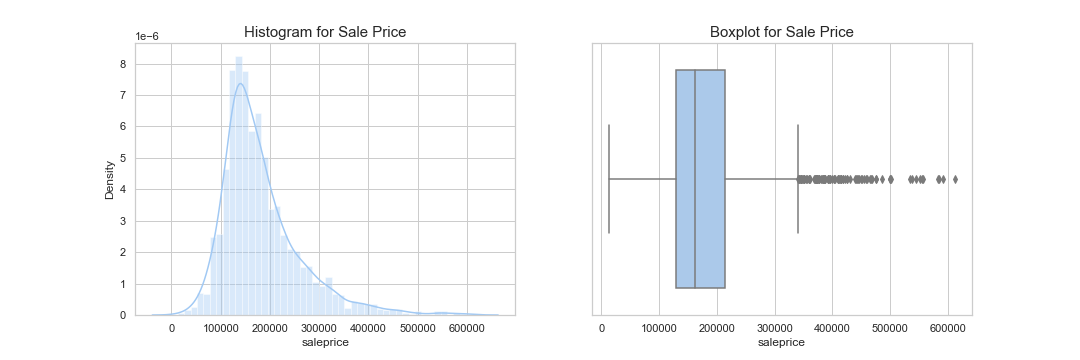
Looking at our target variable, it is right-skewed and many outliers have been detected by the boxplot. There are no null values, so we won’t have to worry about using it in our model.
Features
Processing and EDA of the variable types were done according to their feature types i.e. Nominal, Ordinal, Continuous and Discrete. The codebook contains the full process of how each variable was evaluated and shortlisted or rejected. Here is a brief overview:
Nominal Any nominal variables we included in our model needed to be one-hot encoded for each category. Hence, we prioritized variables that have a clear impact on the sale price, looping through the variables to calculate the correlation and record one-hot encoded variables that fulfill the following:
- They had more than an absolute value of 0.3
- They constitute more than 5% of the total entries
1
2
3
4
5
6
7
8
9
10
11
12
13
14
15
16
17
18
19
20
# Code to shorlist nominal features (the variable nominal is a list consisting of all names of nominal features)

nominal_dummies = []
for var in nominal:
    value_c = df[var].value_counts(normalize=True).sort_index() #Get the normalized value counts for the variable
    dummy_df = pd.get_dummies(df[var],prefix=var) #One-hot encode variable
    dummy_df = dummy_df.join(df['saleprice']) #Add sale price to one-hot encoded values
    dummy_corr = dummy_df.corr(method='spearman') #Calculate correlation for one-hot encoded values with saleprice
    for i, value in enumerate(dummy_corr['saleprice']): #Loop through saleprice correlations to check for suitable nominal variables
        variable_cat = dummy_corr.index[i]
        if var != 'saleprice' and variable_cat != 'saleprice': #Rule out saleprice correlation (will be 1.0)
            counts = value_c[i]
            if abs(value) >= 0.3 and counts >= 0.05: #Check to see if correlation is more than 0.3 and value counts are sufficient
                entry = {}
                entry['variable'] = var
                entry['var_category'] = variable_cat
                entry['correlation'] = value
                entry['value_counts'] = counts
                nominal_dummies.append(entry) #Add dictionary for variable category to our list
We also looked at the boxplots for each of the nominal variables.
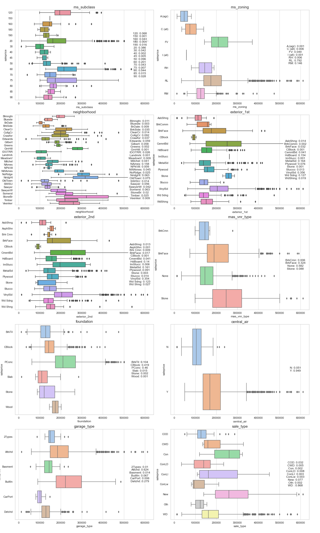
Looking at the boxplots and nominal_corr_df table, we can see that for the variables identified with higher correlations, we can see some differentiation in terms of sale price values.
Ordinal
Ordinal variables had to be first mapped to numerical values. For example:
1
2

df['exter_qual'] = df['exter_qual'].map({'Po':1,'Fa':2,'TA':3,'Gd':4,'Ex':5})
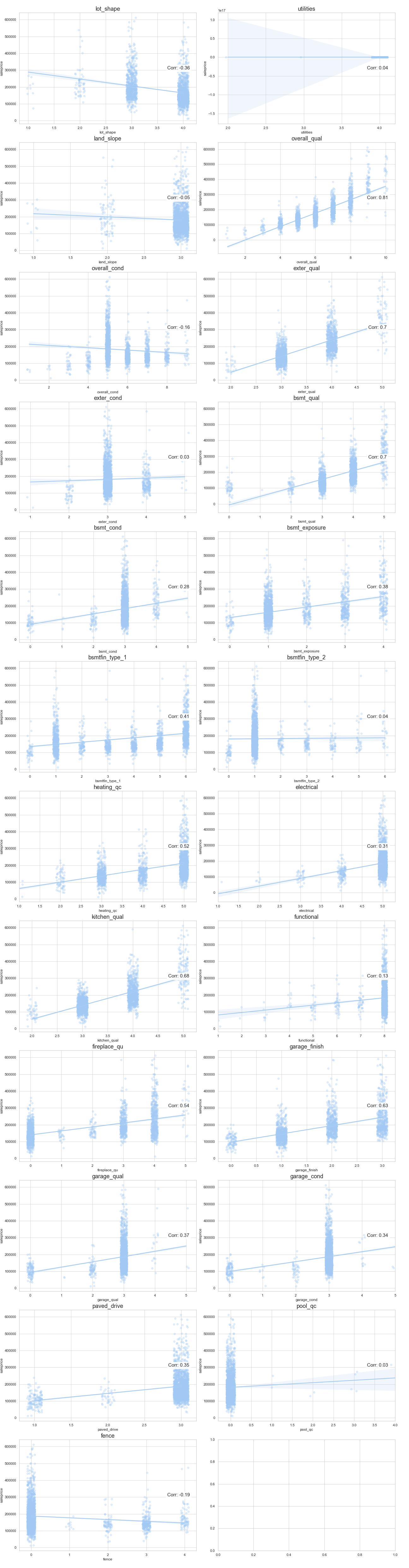
Based on the plots and correlation scores, these features were shortlisted:
1
2
3
4
5
6
7
8
9
10
11
12
13
'overall_qual',
 'exter_qual',
 'bsmt_qual',
 'bsmt_exposure',
 'bsmtfin_type_1',
 'heating_qc',
 'electrical',
 'kitchen_qual',
 'fireplace_qu',
 'garage_finish',
 'garage_qual',
 'garage_cond',
 'paved_drive'
The discrete and continuous features were also evaluated according to boxplot and correlation scores, where we also combined certain features e.g. house age by subtracting the year built from the year sold.
2. Modeling & Tuning
We split our data into a train and test validation set before proceeding with the modeling. The Linear Regression, Lasso and Ridge models were tested on the data, where we also used PolynomialFeatures to combine our top-performing features.
These features were then reduced to 30 features with the use of RFE (Recursive Feature Elimination).
The model was evaluated by submitting a csv submission to kaggle, which scores the data on mean squared error.
The final model selected was a ridge model with a private and public score of 30,027 and 28,062 respectively, which is relatively better compared to the baseline model’s score around 80,000.
3. Interpretation
To evaluate our model, we look at the residual error of the predicted values (this is validated on our test dataset that was created initially).
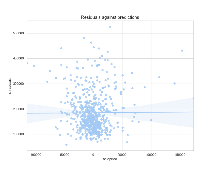
It looks like as sale price increases, we tend to get a higher range of error. This indicates that the model may not be as useful for predicting sale price beyond a certain number, where other factors not available in the dataset may be affecting the target.
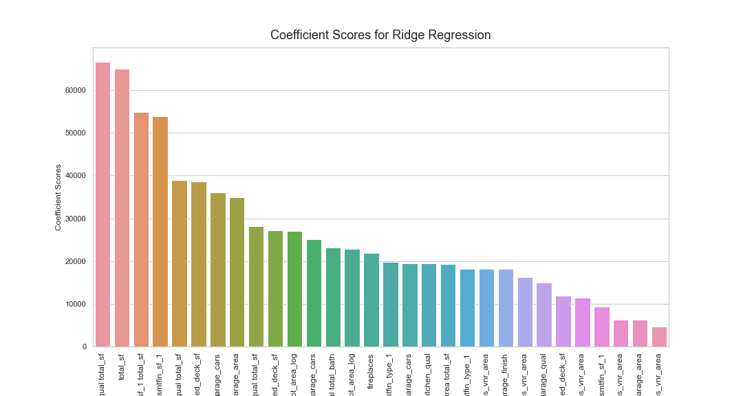
We can see that the features with the top 3 highest coefficient scores are all features based on total_sf. This feature continues to show up in the other coefficients, and is in 50% of our top 10 features. Interestingly, this variable was created from other square-foot values in the dataset, which shows us the importance of feature engineering.
Conclusion & Recommendations
We have successfully built a model with a relatively good RMSE based on the training dataset provided, and our examination has indicated that while the top influencing factor appears to be area (total square feet of the house and individual areas), variables across different aspects of the house were also picked out by the model to be significant.
Recommendations
If we had additional time and resources, we may want to consider the following to improve on and continually iterate on our model:
-
The frequency distribution of the log of sale prices follows a normal distribution. By building our linear regression model with the log of sale prices, we can better fit and predict the sale prices of houses in the higher price range.
-
For features with many different categories, we can combine and regroup them so that each category becomes more significant. For eg: Neighborhood has 28 categories, we can regroup them into 5 categories based on their mean sale prices.
-
We can also look into other external factors affecting housing prices like economic factors and demographic data of the community.
While we see that the model built has limitations, it is also true that the process of putting together the model is informative and a similar process can be conducted for other datasets in other cities or with different variables collected. Our process is as follows:
- Clean and process data
- Exploratory data analysis
- Feature engineering
- Feature selection (by judgement and RFE and lasso techniques)
- Model iteration and optimisation
The last step should be ongoing if there is a stream of new data. Any model will have its limitations, but with the right set of assumptions and understanding of suitable use cases, we’re able to predict meaningfully.